Just recently, I had my very first experience working with Amazon Athena (Athena). Athena is an interactive query service that makes it easy to analyze data in Amazon Simple Storage Service (Amazon S3) using standard SQL. In simpler terms, Athena lets SQL run queries against data stored in Amazon S3 without actually having any database servers.
First, I explored the basics of Athena, like creating logical databases and tables against which we can run queries. Then I realized that, when optimizing for performance and cost, it is crucial to be specific in how we define the tables, databases, and folder structures stored in Amazon S3.
We will use a sample stock market dataset from the past 20 years to illustrate these optimizations, which we also utilized in a related PoC, Rapid Data Lake Development with Data Lake as Code Using AWS CloudFormation. In addition to the sample stock market dataset, we’re also going to use another PoC because of the dataset’s volume and rapid growth potential.
The dataset
After getting the sample data, we will need to stage it in Amazon S3 and look at how the files are structured. First, we put the data in Amazon S3 using a bucket called s3://nclouds-datalake-stockmarket
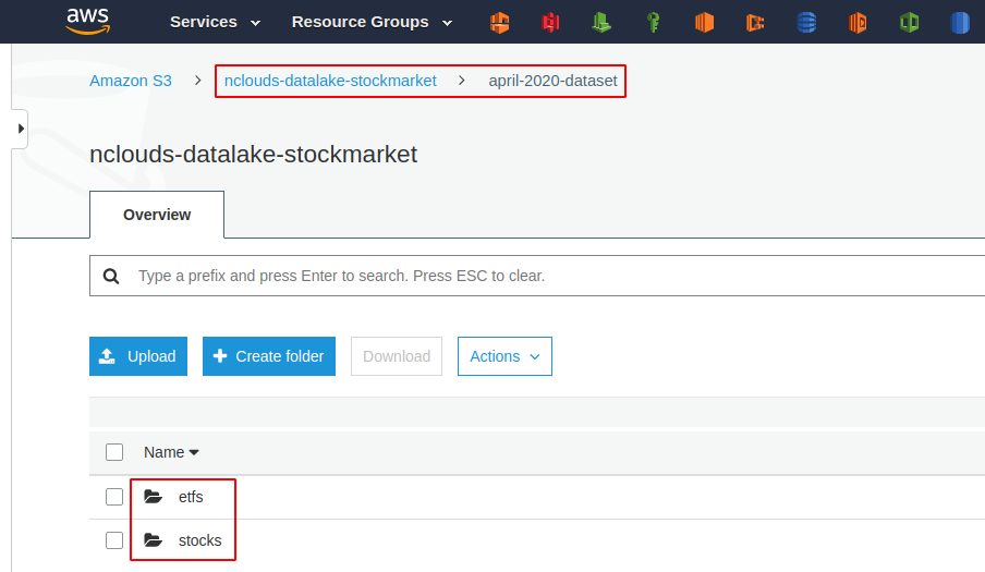
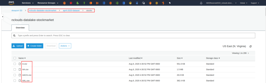
At the first level, we see a folder called april-2020-dataset. There are two folders on the second level — one folder for stocks and one for Exchange Traded Funds (ETFs). Inside the stock and ETF folders, we see one file per ticker symbol. Each file includes information about every specific stock and ETF.
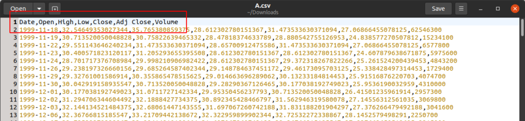
Now, let’s take a look at the data inside these files. After opening a random file, we see the following columns: Date, Open, High, Low, Close, Adj Close, Volume. We also know that all of these files will have the same structure. With this information, we can begin creating resources in Athena and running queries.
Amazon Athena
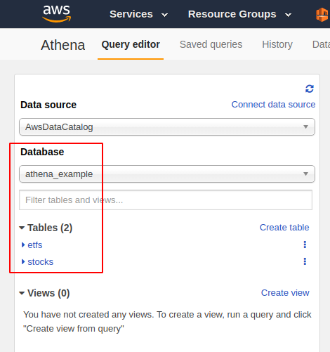
We begin by creating two tables in Athena, one for stocks and one for ETFs. Both tables are in a database called athena_example. To create these tables, we feed Athena the column names and data types that our files had and the location in Amazon S3 where they can be found. The table path for the stocks is s3://nclouds-datalake-stockmarket/april-2020-dataset/stocks. The table path for the ETFs is s3://nclouds-datalake-stockmarket/april-2020-dataset/etfs.
Now let’s try a query — the top ten highest closing prices for December 2010.
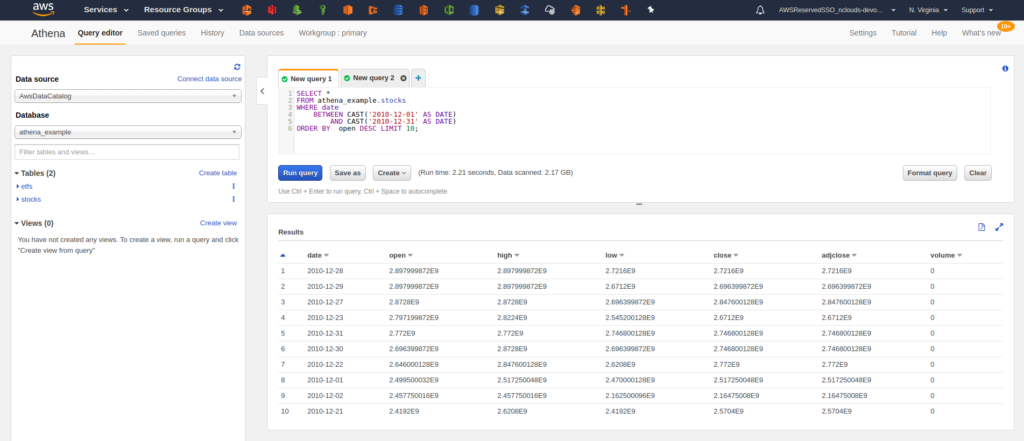
We can query our files in Amazon S3 directly from Athena, and now we see results from both queries. However, there is a problem. Our query worked, but now we can’t tell which stock or ETF those prices belong to. Why? Because Athena is not picking up that information. The ticker symbols for the stocks and ETFs are the names of the files in Amazon S3. The way it is set it up is resulting in those values being lost. To fix this, we’ll use table partitioning.
Table partitioning
We have a problem with our Athena tables — there’s no correlation between the stock and ETF symbols with tabular values (i.e., due to the structure of the raw data). We’ll fix this problem by partitioning our data to include the ticker symbol information currently stored in each file’s name. We can also add an extra column, ‘type,’ that will allow us to store everything in a single table and still be able to differentiate between stocks and ETFs.
To create these two ‘type’ and ‘ticker’ partitions, we need to make some changes to our Amazon S3 file structure. I wrote a small bash script to take the original bucket’s data and copy it into a new bucket with the folder structure changes. Once that’s done, the data in Amazon S3 looks like this:
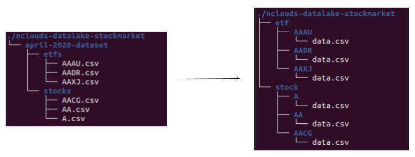
Now we have a folder per ticker symbol. Inside each folder, we have the data for that specific stock or ETF (we get that information from the parent folder). We can create a new table partitioned by ‘type’ and ‘ticker.’
The new create table command in Athena is:
CREATE EXTERNAL TABLE `partitioned`(
  `date` date,
  `open` double,
  `high` double,
  `low` double,
  `close` double,
  `adjclose` double,
  `volume` bigint)
PARTITIONED BY (
  `type` string,
  `ticker` string)
LOCATION
  's3://nclouds-datalake-stockmarket-partitioned/'
If we query this table now, you’ll notice that, while we don’t get any errors, we also don’t get any results. That’s because this new table is partitioned, and we need to tell Athena where it can find those partitions. It’s possible to do that through an AWS Glue crawler, but in this case, we use a Python script that searches through our Amazon S3 bucket folders and then creates all the partitions for us. For this use case, our partitions are all possible combinations of ‘type’ and ‘ticker.’ Once those are created, you will see them in the AWS Glue console.
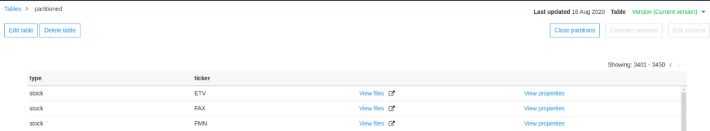
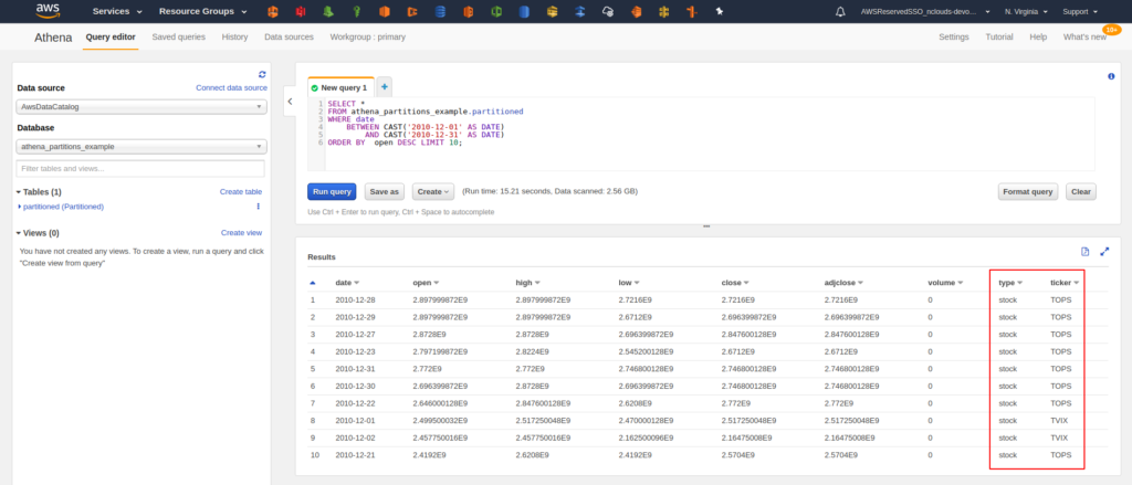
Now that we have defined our partitions, we can run the previous query and check the new results. We see two new columns that correspond to the two partitions we created.
Partitioning and cost optimization
You might be wondering how properly partitioning your tables helps with cost optimization. To understand this, we need to know what AWS charges for Athena queries based on the amount of data it scans from Amazon S3. The current price is $5 for every 1TB of data scanned. That being the case, we need to make sure that Athena scans the least amount of data possible so that our queries run faster, which optimizes costs. That’s one cost savings benefit of partitions that’s often overlooked.
Let’s take a look at the previous query. This time, let’s focus on the amount of data that was scanned from Amazon S3.
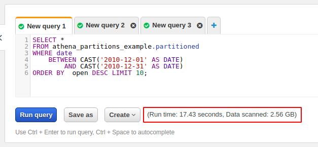
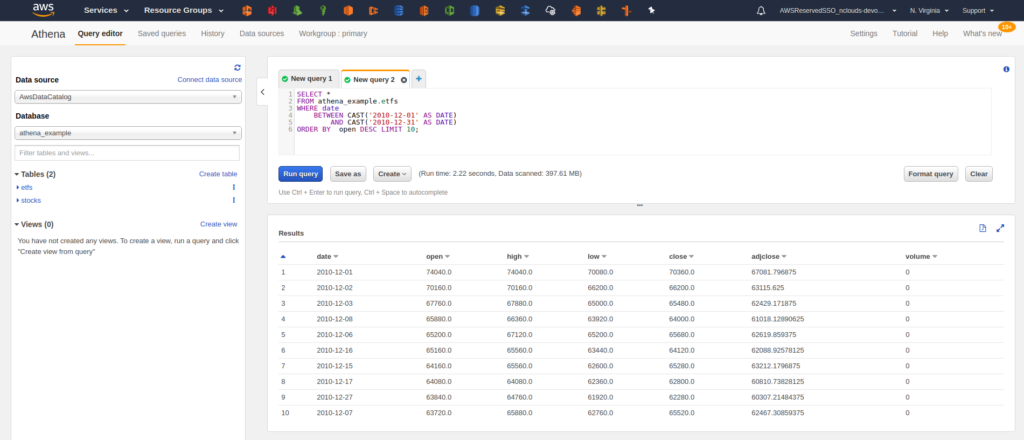
On this query, we were looking for the top ten highest opening values for December 2010. That query took 17.43 seconds and scanned a total of 2.56GB of data from Amazon S3. Without partitions, roughly the same amount of data on almost every query would be scanned. But, thanks to our partitions, we can make Athena scan fewer files by using Amazon S3. For example, let’s run the same query again, but only search ETFs.
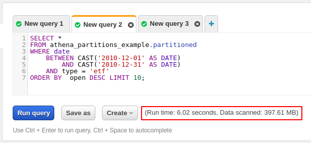
You see that this time the query took only 6.02 seconds, and it scanned only 397.61MB due to our folder structure. If we use a condition like “type=etf,” Athena has to scan only the ‘etf/’ folder in our bucket. Let’s drill down a bit more and add one more condition to our query that will search ‘ticker=SOXS.’
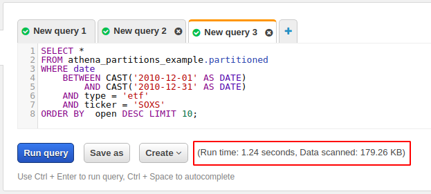
This time the scan took only 1.24 seconds and scanned merely 179.26KB of data. That’s a super cheap query.
In conclusion
Creating partitioned tables is one of the best ways to write more cost-efficient queries. Other factors that may help boost performance while reducing costs are minimizing the amount of nesting in queries, selecting necessary columns vs. all columns (i.e., SELECT *), and using the WITH clause in Athena if you need to use nested queries. If our data is structured correctly, we can design more complete tables, which allows us to be more specific when writing queries. If we use the right condition statements, we can avoid directing Athena to scan unnecessary files and eliminate extra costs.
Need help with Amazon Athena or your overall data and analytics strategy? We’ve got the experience, AWS data and analytics how-to knowledge, plus our own research initiatives, to help you plan and execute your strategy.